Pearson Correlation Calculator
Quantify linear relationships with mathematical certainty. Calculate correlation coefficients, p-values, and covariance with our advanced statistical engine.
Pearson Correlation Calculator
Enter your data points to calculate the Pearson correlation coefficient. Get r, r-squared, p-values, and step-by-step solutions instantly in your browser.
Enter your data points
| # | X Values | Y Values |
|---|
Results
Pearson Correlation (r)
R-Squared (r²)
P-value
Regression Slope (from r)
Strength
Direction
Std. Dev. of X (sₓ)
Std. Dev. of Y (sᵧ)
Mean of X
Mean of Y
Covariance
Data Points (n)
Remember: Correlation does not imply causation. A significant correlation only indicates association, not that one variable causes the other.
Step-by-Step Solution
How to Use This Pearson Correlation Calculator
Measure Correlation
Computes the Pearson r coefficient between two continuous variables.
Enter X & Y Pairs
Input paired numeric data as comma-separated values in two columns.
Full Analysis
Get r, R², p-value, covariance, and a step-by-step breakdown.
Best For
Testing linear relationships in research, finance, and social sciences.
Pearson r only measures linear association — use a scatterplot first to check for non-linear patterns.
What Is the Pearson Correlation Coefficient?
The Pearson correlation coefficient (r) measures the strength and direction of the linear relationship between two continuous variables. It ranges from −1 (perfect negative correlation) to +1 (perfect positive correlation), with 0 indicating no linear relationship.
Unlike regression, which predicts one variable from another, correlation simply quantifies how closely two variables move together. Named after the British statistician Karl Pearson who developed the modern formulation in the 1890s, building on earlier work by Francis Galton on regression and correlation in heredity studies, the Pearson r remains the most widely used measure of association in statistics.
The coefficient is dimensionless — it has no units — which makes it convenient for comparing relationships across different variables measured on entirely different scales. When r is close to +1, the two variables increase together in near-perfect lockstep; when r is close to −1, one variable rises as the other falls; and when r is near 0, there is little to no linear association.
Importantly, r only captures linear relationships — two variables can have a strong nonlinear relationship (such as a U-shape) and still yield r ≈ 0. For this reason, always inspect a scatter plot before relying on the numerical value of r. The squared correlation r² (called the coefficient of determination when used in regression) tells you the proportion of shared variance between the two variables: if r = 0.8, then r² = 0.64, meaning 64% of the variability in one variable can be linearly accounted for by the other.
Pearson's r is symmetric, meaning r(X,Y) = r(Y,X) — the correlation between height and weight is the same whether you treat height or weight as the first variable. This symmetry distinguishes correlation from regression, where regressing Y on X produces a different line from regressing X on Y (unless r = ±1). The population parameter is denoted ρ (rho), and the sample statistic r is an estimate of ρ.
As the sample size increases, r converges toward the true population correlation, making larger samples more reliable for estimating the strength of association.
Pearson Correlation Formula Calculator Explained
The Pearson correlation coefficient is defined as the ratio of the covariance of X and Y to the product of their standard deviations. In terms of sums of squares, the formula is r = SSxy / √(SSxx × SSyy), where SSxy = Σ(xᵢ − x̄)(yᵢ − ȳ) is the sum of cross-products (also called the corrected covariance sum), SSxx = Σ(xᵢ − x̄)² is the sum of squared deviations of X, and SSyy = Σ(yᵢ − ȳ)² is the sum of squared deviations of Y.
An equivalent expression using the covariance and standard deviations is r = sxy / (sx × sy), where sxy = Σ(xᵢ − x̄)(yᵢ − ȳ) / (n − 1) is the sample covariance, and sx and sy are the sample standard deviations of X and Y respectively.
The covariance sxy captures how X and Y vary together: positive values indicate that above-mean X values tend to pair with above-mean Y values, while negative values indicate the opposite. However, covariance alone depends on the units of measurement — a covariance of 500 in one dataset may represent a weaker association than a covariance of 5 in another if the scales differ.
Dividing by the product of the standard deviations normalizes this measure, forcing the result into the range [−1, +1] regardless of the original units. This normalization is what makes Pearson's r so universally applicable and comparable across studies.
A third equivalent formula using raw sums (no deviation scores) is r = [nΣxy − ΣxΣy] / √{[nΣx² − (Σx)²][nΣy² − (Σy)²]}, which is computationally convenient for hand calculation or spreadsheet implementation because it avoids computing means and deviations separately. Our calculator displays both the deviation-score and raw-sum approaches in its step-by-step solution so you can follow whichever formulation you prefer.
Understanding that all three forms are mathematically equivalent is important for building confidence in the calculation and for recognizing the formula in different textbook presentations. The covariance approach provides the most intuitive understanding of what r measures: it captures the degree to which two variables co-vary (move together) relative to how much each varies on its own.
When the cross-products SSxy are large relative to both SSxx and SSyy, it means that points that deviate far from the mean in X also tend to deviate far from the mean in Y in the same direction (for positive r) or the opposite direction (for negative r).
When the cross-products are small relative to the individual deviations, it means that knowing how far X is from its mean tells you little about how far Y is from its mean, resulting in r close to zero.
| Component | Symbol | Description |
|---|---|---|
| Covariance | sxy | Sum of cross-products divided by (n-1) |
| Std Dev X | sx | Square root of sum of squared X deviations |
| Std Dev Y | sy | Square root of sum of squared Y deviations |
| Correlation | r | Covariance divided by product of standard deviations |
| R-squared | r squared | Proportion of shared variance |
| p-value | p | Statistical significance of r |
How to Interpret Pearson's r
|r| ≥ 0.9 — Very Strong correlation
0.7 ≤ |r| < 0.9 — Strong correlation
0.5 ≤ |r| < 0.7 — Moderate correlation
0.3 ≤ |r| < 0.5 — Weak correlation
|r| < 0.3 — Very Weak or No correlation
Understanding the p-Value in Correlation
The p-value answers a critical question: if the true population correlation were actually zero, how likely is it that we would observe a sample correlation as extreme as the one we calculated? A small p-value (typically < 0.05) means that such an extreme r would be very unlikely under the null hypothesis, so we reject the null hypothesis and conclude that the correlation is statistically significant — that is, it is unlikely to be a chance finding.
A large p-value means the observed r could plausibly have arisen by chance even if no true correlation exists, so we cannot confidently claim a real association. The standard significance levels are α = 0.05 (5% chance of a false positive), α = 0.01 (1% chance), and α = 0.001 (0.1% chance).
The p-value depends heavily on the sample size: with n = 5, even r = 0.87 may not be significant (p > 0.05), whereas with n = 100, r = 0.20 can be highly significant (p < 0.05). This means that statistical significance and practical significance are different concepts — a tiny r can be statistically significant with enough data, while a large r can be non-significant with too few data points.
Always consider both the magnitude of r and the p-value together, along with the sample size and the practical context of the research question. Our calculator computes the exact p-value using the t-distribution with n − 2 degrees of freedom, which is the standard approach for testing H₀: ρ = 0. The p-value is determined by comparing the t-statistic t = r√(n − 2) / √(1 − r²) against the t-distribution.
When reporting results, it is best practice to report the exact p-value rather than simply stating "significant" or "not significant" at a particular threshold, because the exact p-value conveys the strength of the evidence against the null hypothesis.
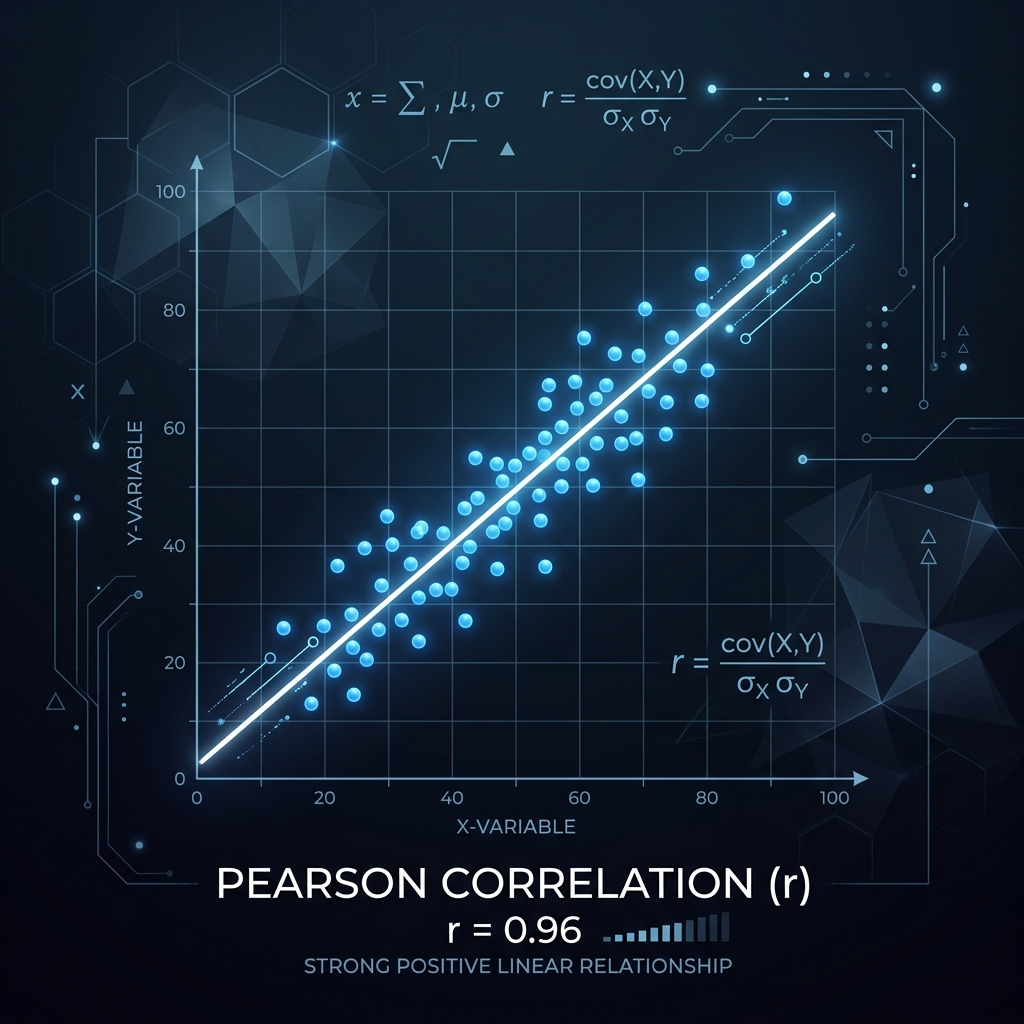
Reading a Scatterplot for Correlation
A scatterplot is the single most important diagnostic tool for correlation analysis. Before computing r, you should always plot your (X, Y) data points to visually assess whether the relationship is linear and whether outliers are present. Here is what to look for: Direction — if the points trend upward from left to right, the correlation is positive; if they trend downward, it is negative; if they form a horizontal cloud, r will be near zero.
Strength — the tighter the points cluster around an imaginary straight line, the closer |r| will be to 1; the more dispersed the cloud, the closer r will be to 0. Linearity — if the points follow a curved pattern (U-shape, exponential, etc.) rather than a straight line, Pearson's r will underestimate the true strength of association because it only measures linear relationships.
In such cases, Spearman's rank correlation or a transformation may be more appropriate. Outliers — a single extreme point far from the main cluster can dramatically inflate or deflate r, pulling the correlation toward or away from zero depending on its position. Always investigate outliers before trusting the numerical result.
Clusters — if the data separates into distinct subgroups, the overall r may be misleading because it mixes different underlying patterns. Consider analyzing each subgroup separately. Heteroscedasticity — if the spread of points widens or narrows across the range of X, the correlation may not adequately describe the relationship at all levels.
Our calculator displays an interactive scatterplot alongside the numerical results so you can immediately verify that the correlation value matches what you see visually. If the scatterplot and the r value seem to disagree, trust the scatterplot — the visual pattern is more informative than any single summary statistic.
When to Use Pearson Correlation
Pearson correlation is the appropriate tool when you need to measure the strength and direction of a linear association between two continuous variables without fitting a predictive model. Use it when both variables are approximately normally distributed, when a scatterplot shows a roughly linear pattern, and when no extreme outliers are present. It is particularly useful for initial exploratory analysis before building a regression model, for assessing test-retest reliability, for checking multicollinearity between predictors, and for validating that an expected relationship actually exists in your data.
Pearson correlation is also the standard method for computing the correlation matrix that underpins principal component analysis, factor analysis, and structural equation modeling. However, remember that correlation does not imply causation — a significant r only tells you that two variables co-vary, not that one causes the other. The table below summarizes common fields where Pearson correlation is applied with concrete examples.
Both variables are continuous (numeric) and approximately normally distributed
The relationship appears linear (check with a scatter plot)
You want to measure association, not predict one variable from another
There are no extreme outliers that could distort the result
Frequently Asked Questions
What is the range of the Pearson correlation coefficient?
The Pearson correlation coefficient r always falls within the range −1 to +1. A value of +1 indicates a perfect positive linear relationship where every data point lies exactly on an upward-sloping line; −1 indicates a perfect negative linear relationship where every point lies on a downward-sloping line; and 0 indicates no linear relationship.
Values close to the extremes represent stronger associations, while values near zero represent weaker ones. The sign indicates direction: positive means both variables increase together, negative means one increases as the other decreases. It is mathematically impossible for |r| to exceed 1 — if your calculation produces |r| > 1, there is a computational error in your work.
Does correlation imply causation?
No. Correlation measures association, not causation. A significant Pearson r only tells you that two variables tend to move together — it does not prove that one causes the other. The observed association could be due to a confounding variable that influences both, to reverse causation (Y causes X instead of X causing Y), or to pure coincidence.
For example, ice cream sales and drowning rates are positively correlated, but eating ice cream does not cause drowning — both increase during warm weather, which is the confounding variable. Establishing causation requires controlled experiments, temporal ordering, and ruling out alternative explanations — not just a high correlation. Always remember: correlation ≠ causation, no matter how strong the correlation appears to be.
What is the difference between Pearson and Spearman correlation?
Pearson's r measures the strength of the linear relationship between two continuous variables, assuming both are approximately normally distributed. Spearman's ρ (rho) measures the strength of the monotonic relationship using the ranks of the data rather than the raw values.
Spearman is preferred when your data has outliers, when the variables are ordinal rather than interval/ratio, or when the relationship is monotonic but not linear (for instance, a curve that consistently rises but at a varying rate). Pearson is more powerful when its assumptions are met, but Spearman is more robust when they are not.
In practice, if Pearson and Spearman give similar results, the relationship is approximately linear; if Spearman is much larger than Pearson, the relationship is likely monotonic but nonlinear, suggesting that a transformation or rank-based method is more appropriate.
How do outliers affect Pearson's r?
Outliers can dramatically distort the Pearson correlation coefficient because the formula squares deviations, giving extreme points disproportionate influence. A single outlier far from the main cluster can inflate r toward +1 or −1 (if the outlier lies along the general trend) or deflate r toward 0 (if the outlier contradicts the trend).
️ For example, in a dataset of 30 points with r = 0.2, adding one extreme point aligned with a positive trend could push r above 0.5 — a completely misleading result. Before computing r, always inspect a scatterplot for outliers. If outliers are present, consider using Spearman's rank correlation (which uses ranks and is resistant to extreme values), robust correlation methods, or removing the outlier if it is a data-entry error. Never report r without first checking for influential observations.
What does a negative Pearson correlation mean?
A negative Pearson r means that as one variable increases, the other tends to decrease — the variables move in opposite directions. For example, r = −0.85 between temperature and heating costs would mean that colder temperatures are associated with higher heating expenses.
The magnitude |r| still indicates strength: r = −0.85 is just as strong as r = +0.85; only the direction differs. A common mistake is treating a negative correlation as a "bad" result — it simply indicates an inverse relationship.
🔍 Negative correlations are common in many fields: price and demand (higher price reduces demand), age and physical flexibility (flexibility tends to decline with age), distance and signal strength (signals weaken with distance), stress and immune function (higher stress correlates with weaker immunity), and unemployment and consumer confidence (unemployment erodes confidence). When you encounter a negative correlation, first verify it makes substantive sense, then interpret its magnitude using the same |r| thresholds you would use for a positive correlation.
How many data points do I need for a reliable Pearson correlation?
The mathematical minimum is 2 data points, but this is meaningless for inference. For a reasonably reliable estimate, aim for at least 10–20 data points.
For significance testing, small samples require very large r values to achieve p < 0.05 — with n = 5, you need |r| > 0.88; with n = 20, you need |r| > 0.44; with n = 50, you need |r| > 0.28. The more data you have, the more precisely you can estimate the true correlation and the smaller a correlation can be while still being statistically significant.
A useful rule of thumb is that you need at least n = 30 for the confidence interval around r to be reasonably narrow, and n = 100 or more for precise estimation of modest correlations around |r| = 0.2.
What is the p-value for Pearson correlation?
The p-value tests the null hypothesis that the true population correlation ρ = 0. It is computed using the t-statistic t = r√(n − 2) / √(1 − r²) with n − 2 degrees of freedom.
A p-value < 0.05 means the observed correlation is unlikely to have occurred by chance alone, so we reject the null hypothesis and conclude the correlation is statistically significant.
However, significance depends heavily on sample size — a small r can be significant with enough data, while a large r can be non-significant with too few observations.
The critical r values for significance at α = 0.05 are approximately: |r| > 0.88 for n = 5, |r| > 0.63 for n = 10, |r| > 0.44 for n = 20, |r| > 0.28 for n = 50, and |r| > 0.20 for n = 100.
This illustrates why you should never rely on p-values alone — always report r, r², the sample size, and ideally a confidence interval alongside the p-value to give a complete picture of the evidence for and against the null hypothesis.
What are the assumptions of Pearson correlation?
Pearson correlation assumes: (1) Linearity — the relationship between X and Y is linear (check with a scatterplot); (2) Normality — both variables are approximately normally distributed (check with histograms or Q-Q plots); (3) Interval/ratio data — both variables are measured on a continuous numeric scale; (4) Homoscedasticity — the variability of Y is roughly constant across the range of X; (5) No extreme outliers — outliers can severely distort r.
If these assumptions are violated, consider using Spearman's rank correlation instead, which is more robust. You can also use our Regression Assumptions Checker to formally test the linearity and normality assumptions on your data.
Can Pearson correlation be used for categorical data?
No. Pearson's r requires both variables to be continuous (interval or ratio scale). If your variables are categorical, use chi-square tests for nominal categories or Spearman's rank correlation for ordinal categories. If you have one continuous and one binary variable, you can use point-biserial correlation, which is mathematically equivalent to Pearson's r and produces the same numerical result when the binary variable is coded as 0 and 1, but its interpretation differs because the binary variable represents group membership rather than a continuous measurement.
For two binary variables, use phi coefficient or Cramer's V instead. For nominal variables with more than two categories, Cramer's V or the contingency coefficient are appropriate. Attempting to compute Pearson's r on truly categorical data (e.g., coding eye color as 1, 2, 3) will produce a meaningless number because the numeric codes are arbitrary and do not represent an ordered scale.
What does r² mean in correlation?
r² (the coefficient of determination) represents the proportion of shared variance between the two variables. If r = 0.7, then r² = 0.49, meaning 49% of the variability in one variable can be linearly accounted for by the other.
This is often more intuitive than r itself because it directly quantifies explanatory power. In regression, r² equals R² from the regression of Y on X — they are the same quantity viewed from different perspectives.
Note that squaring r always reduces the apparent strength: r = 0.5 means only 25% shared variance, which is often weaker than people expect. This is why a correlation of 0.3, while sometimes called "weak," actually explains less than 10% of the variance (r² = 0.09) — it is far weaker than the raw r value might suggest. The relationship between r and r² is nonlinear: doubling r from 0.5 to 1.0 quadruples r² from 0.25 to 1.0.
Always report both r and r² so readers can assess both the direction and the practical importance of the association.
Is a correlation of 0.5 strong or weak?
It depends on the context. By conventional guidelines, r = 0.5 is moderate — not weak, not strong. In psychology and social sciences, r = 0.5 may be considered quite respectable because human behavior is inherently variable and rarely produces correlations above 0.7.
In physics or engineering, where relationships are expected to be near-deterministic, r = 0.5 might be considered disappointingly low. Always interpret the magnitude of r relative to what is typical in your specific field, and always report r² alongside r so readers can judge the proportion of shared variance.
Remember that r = 0.5 means only 25% shared variance (r² = 0.25) — the remaining 75% of the variability is due to other factors or random noise. This often surprises people who expect r = 0.5 to represent a "half-strength" relationship.
Can I use Pearson correlation on non-normal data?
Pearson's r can be calculated on any two continuous variables, but the p-value and inference rely on approximate normality. With large samples (n > 30 per variable), the central limit theorem provides some protection, and the p-value is fairly robust to mild non-normality. With small samples or severely non-normal data (heavy skew, extreme outliers), the p-value may be unreliable and the confidence intervals inaccurate.
In such cases, consider Spearman's rank correlation (which does not assume normality) or a bootstrap confidence interval for r. Always check normality with a histogram or Q-Q plot before trusting the p-value from small samples. The point estimate of r itself is always valid regardless of normality — it is only the significance tests and confidence intervals that depend on the distributional assumption.
What is the difference between correlation and regression?
Correlation measures the strength and direction of the linear association between two variables, producing a single number r between −1 and +1. Regression goes further by fitting a predictive equation ŷ = mx + b that allows you to estimate Y from X. Correlation is symmetric (r(X,Y) = r(Y,X)), while regression is not (regressing Y on X gives different results from regressing X on Y, unless r = 1).
The slope of the regression line is related to r by the formula m = r · (sy / sx). Use our Pearson calculator when you only need to measure association; use a regression calculator when you need to predict Y from X. In practice, the two analyses complement each other — compute r first to check whether a meaningful linear association exists, then build a regression model if prediction is your goal.
How do I report Pearson correlation results?
The standard format is: r(df) = value, p = value. For example, r(28) = 0.72, p = .001. Always include the degrees of freedom (n − 2), the r value to two decimal places, and the exact p-value (or p < .001 for very small values). In APA style, report r with its confidence interval when possible.
Also include a scatterplot to visually support the finding, and note the sample size. Never report r without context — a correlation of 0.6 with n = 8 is far less convincing than 0.6 with n = 200. Best practice is to report the correlation coefficient, the sample size, the p-value, the confidence interval, and a visual plot together so readers can fully evaluate the strength and reliability of the association.
What is a confidence interval for Pearson's r?
A confidence interval for r gives a range of plausible values for the true population correlation ρ. Because r is bounded between −1 and +1 and its sampling distribution is skewed unless ρ = 0, the standard approach uses Fisher's z-transformation: z = 0.5 · ln[(1+r)/(1−r)], compute the CI on z (which is approximately normal with standard error 1/√(n−3)), then transform back to r using r = (e2z − 1)/(e2z + 1).
For example, with r = 0.6 and n = 30, the 95% CI might be approximately (0.30, 0.79). A wide interval indicates low precision (often due to small sample size); if the interval includes zero, the correlation is not statistically significant at that confidence level. Reporting confidence intervals alongside r is strongly recommended by most statistical guidelines because they convey the uncertainty in the estimate far more informatively than a p-value alone.
Can Pearson correlation detect nonlinear relationships?
No. Pearson's r only measures linear association. Two variables can have a perfect nonlinear relationship (such as Y = X² for X in [−5, 5]) and still yield r ≈ 0 because the positive and negative deviations cancel out. If your scatterplot shows a curved pattern, Pearson's r will underestimate the true strength of association.
Use Spearman's rank correlation to detect monotonic nonlinear relationships, or transform the data (e.g., take logarithms or square one variable) before computing r. For more complex patterns such as U-shaped or cyclical relationships, consider polynomial regression or specialized nonlinear models. Always plot your data first — r alone can miss important patterns that are clearly visible on a scatterplot.
What is the difference between Pearson and point-biserial correlation?
Mathematically, point-biserial correlation is identical to Pearson's r — it is simply Pearson's r applied when one variable is continuous and the other is dichotomous (binary, coded as 0 and 1). The formula produces the same numerical result as the standard Pearson calculation.
The difference is purely in interpretation: with point-biserial correlation, r² tells you how much of the continuous variable's variance is explained by group membership, and the sign of r indicates which group (0 or 1) has the higher mean on the continuous variable.
🧮 Point-biserial correlation is commonly used in psychometrics for item-total correlations, in medicine for comparing a biomarker across two diagnostic groups, and in A/B testing for measuring the effect of a binary treatment on a continuous outcome. Our Pearson calculator can compute point-biserial correlation directly — just code your binary variable as 0 and 1.
What is a partial correlation?
Partial correlation measures the linear relationship between two variables after removing the effect of one or more control variables. For example, the partial correlation between salary and education controlling for years of experience tells you whether salary and education are still associated after accounting for the fact that more-educated people also tend to have more experience. The formula for one control variable Z is rxy·z = (rxy − rxz·ryz) / √[(1−rxz²)(1−ryz²)].
Partial correlation is essential when confounders might create a spurious association between X and Y, which is a very common situation in observational research. Higher-order partial correlations control for two or more variables simultaneously and are computed via regression residuals. Many statistical software packages compute partial correlations automatically; our calculator currently computes the standard (zero-order) Pearson r without adjustment for control variables.
If you need partial correlations, you can compute them manually using the formula above along with the pairwise Pearson correlations from our calculator.
Why is my Pearson correlation significant but small?
A small |r| can be statistically significant when the sample size is large. With n = 500, even r = 0.09 yields p < 0.05. This is a common source of confusion: statistical significance means the correlation is unlikely to be zero, not that it is large or important. With enough data, even trivially small correlations become significant.
Always consider practical significance alongside statistical significance — an r of 0.09 explains less than 1% of the variance (r² = 0.008), which is rarely useful in practice regardless of the p-value. Report effect sizes (r and r²) and confidence intervals, not just p-values. A good practice is to ask: "Would this correlation matter in the real world?" If r² is below 0.01, the association may be statistically real but practically negligible.
Can I use this calculator for homework?
Absolutely! This calculator is designed to be an educational tool that helps you learn statistics, not just get answers. It provides complete step-by-step solutions showing every intermediate calculation — the means, deviations, cross-products, and the final r value — so you can follow along, verify your manual work, and understand the mathematical process.
Use it to check your homework answers, study for exams, or learn how to compute Pearson's r by hand. Many instructors encourage using calculators to verify results — just make sure you also understand the underlying concepts and can replicate the steps on your own. The step-by-step output is especially helpful for understanding how deviations from the mean are calculated, how cross-products capture co-variation, and how the normalization by standard deviations produces the final correlation coefficient.
Related Regression Calculators
Discover more specialized regression modeling tools.
Ready to model the trend? Use our regression equation calculator with steps to find the line of best fit.