
Linear Regression Vs Polynomial Regression
Linear regression fits a straight line to data points; polynomial regression fits a curve. Learn the key differences, when to use each, and how to avoid overfitting in this complete guide.
Introduction
Linear regression predicts a dependent variable by fitting a straight line through data points, and polynomial regression predicts it by fitting a curved line that adds squared, cubed, and higher power terms. The choice between the two — model selection — determines whether a model captures a real trend or distorts it.
Each method offers clear benefits. Linear regression produces a simple, interpretable equation with coefficients that are easy to explain. Polynomial regression produces a higher R-squared value on curved data and delivers stronger predictive modeling in nonlinear real-world applications.
A straight line needs only a slope b₁ and an intercept b₀.
Degree n adds one coefficient per power, from x² up to xⁿ.
Both models report the same fit metric, so comparison stays fair.
Both methods share the same components: a dependent variable, predictor coefficients, a fitted equation, and an R-squared value that measures how well the model explains the data. Both are used for forecasting, economics, engineering, and curve fitting. The degree of polynomial, the quality of the fit, and the risk of overfitting decide which method belongs in a given analysis. This guide covers the assumptions of regression, the key differences between the two models, and the common mistakes that follow each.
Understanding Linear Regression
Linear regression models the relationship between a dependent variable and an independent variable by fitting a straight line through the data points. The method assumes that each one-unit increase in x produces a constant change in y, so the entire relationship reduces to two numbers: a slope and an intercept.
The Mathematical Formula
The simple linear regression equation is:
Where:
- y is the dependent (response) variable.
- x is the independent (predictor) variable.
- b₁ is the slope — the change in y for every one-unit increase in x.
- b₀ is the intercept — the predicted value of y when x equals zero.
The least squares method finds the values of b₀ and b₁ that minimize the sum of squared residuals. You can see every calculation step in our step-by-step guide to simple linear regression or run the numbers instantly with the regression equation calculator.
Assumptions of Regression
Linear regression produces valid results only when four assumptions hold. Each assumption protects a different part of the model, from the shape of the fit to the reliability of the p-values.
1. Linearity
The relationship between x and y follows a straight line. Curvature in the data violates this assumption.
2. Independence of Errors
Residuals do not depend on each other. Time-series data often breaks this rule.
3. Homoscedasticity
Residual variance stays constant across all predicted values. A funnel shape signals a violation.
4. Normality of Residuals
Residuals are approximately normal, which keeps p-values and confidence intervals valid.
You can check these conditions automatically with the regression assumptions checker.
Limitations
The main limitation of linear regression is that a straight line cannot represent curvature. When the true relationship bends — such as diminishing returns or accelerating growth — the linear model systematically over-predicts in some ranges and under-predicts in others. This misalignment shows up as a pattern in the residual plot, not as random scatter.
Examples of Use Cases
Linear regression works well in real-world applications with steady, additive relationships:
- Predicting sales revenue from advertising spend.
- Estimating exam scores from hours of study.
- Forecasting energy costs from outdoor temperature.
- Modeling crop yield from rainfall.
In each case, an increase in x moves y by a roughly constant amount, which is exactly what a straight line describes.
The Core Idea
Linear regression turns a cloud of data points into one predictable rule: two coefficients, one straight line. When that line fails to track a bend in the data, the next step is to let the model curve — and that is where polynomial regression begins.
Understanding Polynomial Regression
Polynomial regression extends linear regression by raising the predictor to higher powers. This lets the model follow curves, so the change in y for a one-unit increase in x is no longer constant.
The Mathematical Formula
The polynomial regression equation with degree n is:
A degree 2 model (quadratic) is:
A degree 3 model (cubic) adds an x³ term. Higher degrees add more bends to the curve. Try the polynomial regression calculator, the quadratic regression calculator, or the cubic regression calculator to fit these models to your own data points.
How to Choose the Degree of Polynomial
Choosing the degree of polynomial is a four-step process. Each step adds information that the previous step cannot provide, so the order matters.
Plot the data first
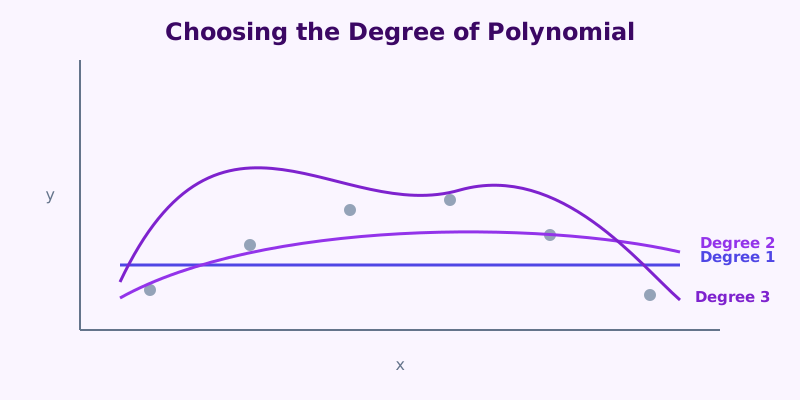
Data visualization is the starting point for model selection. Count the visible bends in the scatter plot — one bend suggests degree 2, two bends suggest degree 3.
Start at degree 1
Fit the linear model first and record its R-squared. This is the baseline every polynomial must beat.
Increase one degree at a time
Add a degree only when it meaningfully improves predictions, not just R-squared. Degrees of 2 and 3 handle most real-world curves.
Validate on new data
Hold out a test set and compare predictive error across degrees. The simplest model with the best out-of-sample performance wins.
Potential Pitfalls: Overfitting
The main risk of polynomial regression is overfitting. A high-degree polynomial passes through nearly every data point, produces a very high R-squared on the training data, and then fails badly on new data. The model memorizes noise instead of learning the underlying trend.
Overfitting Example
A degree 10 polynomial can achieve R² ≈ 1 on 11 data points by wiggling through every point. Apply that same model to new data and the predictions are often useless. A degree 2 model may show R² = 0.85 and generalize far better.
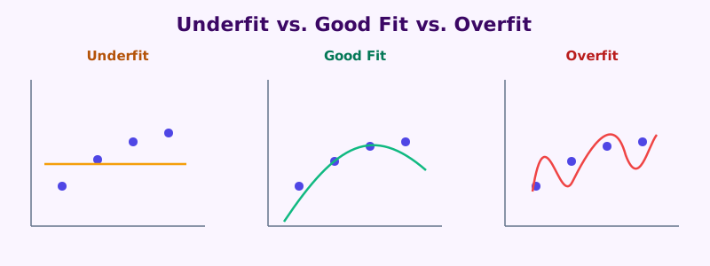
The spectrum of fit quality shows the trade-off. A degree 1 line underfits curved data, a degree 2 curve follows the shape without chasing noise, and a high-degree curve overfits by bending around individual data points. Keep the degree of polynomial as low as the data allows. If a degree 2 or degree 3 model explains the pattern, a higher degree adds complexity without adding value.
Key Differences Between Linear and Polynomial Regression
The differences between the two models come down to flexibility, complexity, and how fit is measured.
Flexibility and Complexity
| Feature | Linear Regression | Polynomial Regression |
|---|---|---|
| Fitted shape | Straight line | Curved line |
| Number of coefficients | 2 (b₀, b₁) | Degree + 1 (b₀ … bₙ) |
| Captures curvature | No | Yes |
| Interpretability | High | Lower at high degrees |
| Risk of overfitting | Low | High with large degree |
Linear regression offers one shape: a straight line. Polynomial regression offers unlimited shapes, one for every degree of polynomial. That flexibility is an advantage on curved data and a liability on noisy data.
Performance Metrics: R-Squared
Both models report an R-squared value, which measures the proportion of variance in y explained by the model. A higher R-squared usually signals a better fit, but the comparison is misleading when degrees differ.
Model explains none of the variation in y.
Every point falls exactly on the fitted line or curve.
Polynomial R² is always equal to or higher than linear R² on the same data.
A high R² alone does not prove a model generalizes.
R-Squared Rule
A polynomial always reaches an R-squared equal to or higher than the linear model fitted to the same data, because a curve can always wrap closer to the data points than a straight line. A higher R-squared alone does not prove the polynomial is the better model — it may just mean the model overfits.
Compare models with predictions on new data, with residual plots, and with degrees kept as low as possible. Statistical significance of each coefficient also matters: a degree 3 term that is not statistically significant should be dropped.
Visual Comparisons
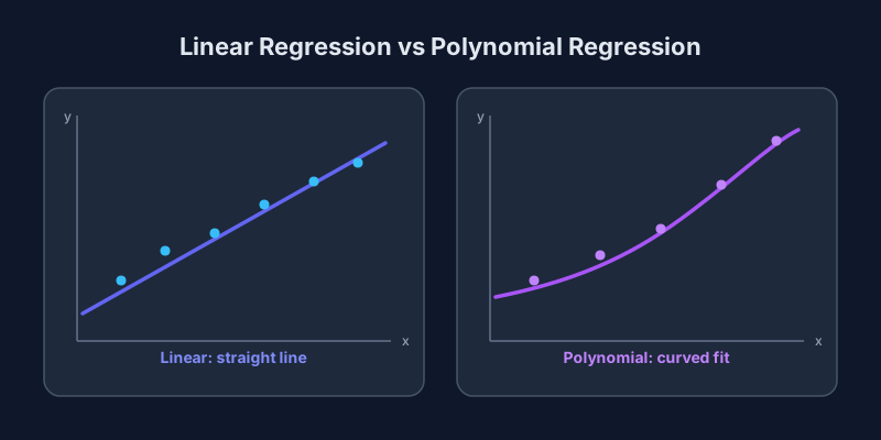
The plot below shows the same set of data points fitted with a straight line and a polynomial curve. The straight line misses the bend in the middle of the data; the curve follows it closely but must be checked for stability beyond the observed range.
Data visualization should always come before model selection. Plot x against y first, look for curvature, and then choose the model that matches the observed shape. A straight line on curved data produces systematic residual patterns; a high-degree curve on linear data produces unstable predictions.
When to Use Each Regression Type
Model selection depends on the shape of the data, the number of data points, and the purpose of the analysis.
Use Linear Regression When
- The relationship between x and y is approximately straight.
- You have fewer than 30 data points.
- You need an interpretable equation for reporting.
- You are extrapolating beyond the observed range, where curves become unreliable.
- Each coefficient must carry a clear real-world meaning.
Use Polynomial Regression When
- The scatter plot shows one or two clear bends.
- You have enough data to support the extra coefficients — at least 10 to 15 points per degree.
- Predictions stay within the observed range of x.
- You want to capture diminishing returns, acceleration, or a U-shaped relationship.
- You have already confirmed the linear model underfits.
The Importance of Data Characteristics
The number of data points and their spread drive the decision. Polynomial regression needs more data because every additional degree consumes degrees of freedom and increases variance. A degree 2 model on 20 points is reasonable; a degree 4 model on 20 points invites overfitting. Data characteristics — sample size, range, and noise — should be assessed before choosing the degree of polynomial, not after.
Common Mistakes and How to Avoid Them
Both model types share failure modes. Most failures trace back to overfitting, underfitting, or skipping validation.
Overfitting and Underfitting
Underfitting happens when a model is too simple for the data — a straight line forced onto curved data produces systematic errors. Overfitting happens when a model is too complex — a high-degree polynomial memorizes noise. The middle ground is a model whose degree matches the true shape of the data and whose coefficients remain statistically significant.
The Importance of Residual Analysis
Residual analysis exposes both problems. Plot residuals against predicted values and read the shape:
Random scatter around zero — the model fits well.
A curved pattern — the model underfits and needs a higher degree or a transformation.
A funnel shape — variance grows with the prediction, violating homoscedasticity.
A few extreme spikes — outliers are pulling the fitted line or curve.
Residual analysis should be a standard step in every regression, not an afterthought. A high R-squared with a patterned residual plot is still a flawed model.
Tips for Validating Models
Validation keeps a good-looking model honest. Follow these five steps in order:
- Hold out a test set — fit on part of the data, then evaluate R-squared and error on the part the model never saw.
- Use cross-validation — repeat the hold-out split several times and average the results.
- Compare against the simpler model — if the polynomial does not beat the linear model on new data, keep the linear model.
- Check each coefficient — drop terms that are not statistically significant.
- Confirm predictions stay in range — never extrapolate a high-degree polynomial beyond the observed data.
The Balanced Model
A good model is the simplest one that explains the data and predicts new data well. If the linear model is nearly as accurate as the polynomial, the linear model is the better choice — less complexity, fewer coefficients, and lower risk of overfitting.
Conclusion
Linear regression fits a straight line and polynomial regression fits a curve, and model selection decides which one belongs in the analysis. Linear regression wins on simplicity, interpretability, and stability; polynomial regression wins on curved data when the degree of polynomial is kept low and the data is large enough to support it.
Use R-squared alongside residual analysis and validation rather than relying on any single metric. Plot the data, start with the simpler model, and add complexity only when the data justifies it. Both methods are worth experimenting with — run the same dataset through the regression equation calculator and the polynomial regression calculator, compare the fitted equations, and check which one predicts new data better. The model that performs well on unseen data, not the model with the highest R-squared, is the one to use.
Try the Polynomial Regression Calculator — It’s Free