
Simple Linear Regression Step-by-Step: The Definitive Mathematical Guide
Learn how to calculate simple linear regression by hand with this 2000+ word walkthrough. Master the slope formula, intercept, R², and residual analysis. Use our regression equation calculator with steps to verify your manual work.
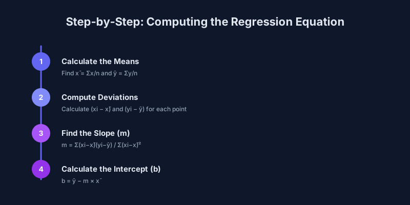
Every statistical journey starts with a single line. Simple linear regression is that line — the most fundamental predictive model in data science, and the foundation upon which every advanced regression technique is built.
If you want to predict a dependent variable from a single independent variable, our free regression equation calculator will give you the answer in seconds. However, understanding how that answer is derived is what separates a data practitioner from someone who merely pushes buttons. For more complex datasets, you might eventually need multiple regression analysis or a broader understanding of regression basics.
What You'll Learn
By the end of this article, you will be able to calculate the regression equation y = mx + b from raw data, interpret the results, and verify that your data meets required assumptions.
Study hours from 2 to 10 with test scores from 65 to 95.
The regression line always passes through the point of means (6.0, 81.0).
Average test score across the five observed students.
What Is Simple Linear Regression?
Simple linear regression models the relationship between one independent variable (x) and one dependent variable (y) by fitting a straight line through the data.
The word “simple” distinguishes it from multiple regression, which uses two or more predictors. The fitted line is chosen to minimize the sum of squared vertical distances — a method called ordinary least squares (OLS).
When to Use (and When to Avoid)
Use It When
- You have one continuous predictor and one continuous outcome.
- Your scatter plot shows an approximately linear pattern.
- You want to quantify how much y changes per unit of x.
Avoid It When
- The scatter plot shows a clear curve — try our quadratic regression calculator instead.
- You have multiple predictors — use multiple linear regression.
- Your data contains extreme outliers that could skew the entire model.
The Dataset
Suppose a tutoring company tracks study hours (x) and resulting test scores (y):
| Student | Study Hours (x) | Test Score (y) |
|---|---|---|
| 1 | 2 | 65 |
| 2 | 4 | 75 |
| 3 | 6 | 80 |
| 4 | 8 | 90 |
| 5 | 10 | 95 |
Step 1: Calculate the Means
The regression line will always pass through the point of means.
Step 2: Compute Deviations and Products
Next, we calculate how far each point is from the mean and multiply the results.
| Student | x − x̄ | y − ȳ | (x − x̄)(y − ȳ) | (x − x̄)² |
|---|---|---|---|---|
| 1 | −4 | −16 | 64 | 16 |
| 2 | −2 | −6 | 12 | 4 |
| 3 | 0 | −1 | 0 | 0 |
| 4 | 2 | 9 | 18 | 4 |
| 5 | 4 | 14 | 56 | 16 |
| Sum | 150 | 40 |
Step 3: Calculate the Slope (b₁)
The slope tells you how much y changes for each one-unit increase in x.
The change in predicted score for every additional hour of study.
For every additional hour of study, the predicted test score increases by 3.75 points.
Step 4: Calculate the Intercept (b₀)
The intercept is the predicted y when x = 0.
The predicted value of y when x equals zero.
A student studying zero hours is predicted to score 58.5.
Step 5: Write the Final Equation
Combining the two: y = 58.5 + 3.75x
This model lets you make predictions. For example, studying for 7 hours yields: 58.5 + 3.75(7) = 84.75.
Extrapolation Danger
Predicting outside your data’s range (e.g., studying 50 hours) is called extrapolation. It often yields nonsensical results and should be avoided.
Step 6: Measure the Fit (R² and r)
R² measures how much of the variation in y is explained by the model. r (Pearson correlation) measures the strength and direction of the linear relationship.
For this dataset, our Pearson correlation calculator would yield an r of 0.9934, which indicates a very strong positive relationship. Learn more about the Pearson Correlation Coefficient on Statology.
Very strong positive linear relationship.
About 98.7% of score variation is explained by study hours.
Each study hour adds 3.75 points to the predicted score.
Five observations; small samples need careful interpretation.
Step 7: Verify Assumptions
Before trusting your results, you must satisfy the four OLS assumptions. Our regression assumptions checker can help you automate this:
1. Linearity
The relationship follows a straight-line pattern.
2. Independence
Observations are not dependent on one another.
3. Homoscedasticity
Residuals (errors) have constant variance.
4. Normality
Residuals are approximately normally distributed.
Beyond Simple Regression
Once you’ve mastered the basics, you might need more advanced tools:
- Multiple Predictors: Use multiple linear regression for complex scenarios.
- Curved Patterns: Use our quadratic regression calculator.
- Growth Models: Explore the exponential regression calculator.
Key Takeaways
The Slope represents the rate of change.
Each extra unit of x changes y by b₁ units — here, 3.75 points per study hour.
The Intercept provides the baseline value at x=0.
A zero-hour student is predicted to score 58.5 points.
R² defines the model’s explanatory power.
R² ≈ 0.987 means the model explains almost all score variation.
Extrapolation is risky — stay within your data’s range.
Predictions outside 2–10 study hours are unreliable.
Correlation is not causation.
Statistics show association, not necessarily cause-and-effect.
Ready to test your own data? Head over to our free regression calculator and get started today!
Deep Dive: Residual Analysis Step-by-Step
Once you have your equation ($y = 58.5 + 3.75x$), the job isn’t finished. You must check the residuals (the errors) to ensure your model is valid.
What is a Residual?
A residual ($e$) is the difference between the observed value ($y$) and the value predicted by your equation ($ŷ$).
Let’s Calculate the Residuals for our Dataset:
| Student | Hours ($x$) | Actual Score ($y$) | Predicted Score ($ŷ$) | Residual ($e$) |
|---|---|---|---|---|
| 1 | 2 | 65 | 58.5 + 3.75(2) = 66.0 | 65 - 66.0 = -1.0 |
| 2 | 4 | 75 | 58.5 + 3.75(4) = 73.5 | 75 - 73.5 = +1.5 |
| 3 | 6 | 80 | 58.5 + 3.75(6) = 81.0 | 80 - 81.0 = -1.0 |
| 4 | 8 | 90 | 58.5 + 3.75(8) = 88.5 | 90 - 88.5 = +1.5 |
| 5 | 10 | 95 | 58.5 + 3.75(10) = 96.0 | 95 - 96.0 = -1.0 |
What to Look for in Residuals:
Sum of Residuals — in OLS regression, the sum should always be zero (allowing for tiny rounding errors). −1.0 + 1.5 − 1.0 + 1.5 − 1.0 = 0.
Randomness — residuals should look like random “noise”. A “U” shape suggests your relationship isn’t linear; consider a quadratic regression calculator.
Outliers — a residual much larger than the others (e.g., 20 in this dataset) indicates an outlier that may be skewing your results.
Confidence Intervals vs. Prediction Intervals
A common point of confusion in our regression equation calculator with steps is the difference between these two intervals.
1. Confidence Interval (for the Mean)
This tells you where the average $y$ for a given $x$ likely falls. Example: “We are 95% confident that the average score for all students who study 6 hours is between 78 and 84.”
2. Prediction Interval (for an Individual)
This tells you where a single new observation likely falls. It is always wider than the confidence interval. Example: “We are 95% confident that John, who studied 6 hours, will score between 70 and 92.”
Frequently Asked Questions (FAQ)
1. Can the slope be negative?
Yes. A negative slope means that as $x$ increases, $y$ decreases. For example, the more miles you drive a car, the lower its resale value. The math remains the same, but your $b₁$ will be a negative number.
2. What if my $x$ and $y$ are swapped?
The regression of $y$ on $x$ is not the same as the regression of $x$ on $y$. Linear regression minimizes the vertical distances ($y$ errors). If you swap them, you are minimizing horizontal distances, which will result in a different equation unless the correlation is perfect (+1 or -1).
3. Why do we square the errors in Least Squares?
- It makes all errors positive (so they don’t cancel out).
- It penalizes large errors more than small ones (a 10-point error is 100 times worse than a 1-point error).
- It makes the math (calculus) easier to solve for a single “best” answer.
4. What is a “good” R² value?
There is no universal “good” value. In a lab experiment, you might want 0.99. In social science, 0.20 might be impressive. What matters more is the context and whether the model helps you make better decisions than a simple average would.
5. Can I use this for non-linear data?
Only if you transform it first. Many researchers take the log of $x$ or $y$ to turn a curve into a line. If the curve is a simple parabola, use a quadratic regression calculator.
6. What is the “Standard Error of the Estimate”?
It’s roughly the average distance that data points fall from the regression line. If your Standard Error is 5, it means your predictions are usually off by about 5 units.
7. How do I know if the slope is “Significant”?
Check the p-value. If the p-value is less than 0.05, we reject the idea that the true slope is zero. This means there is likely a real relationship between $x$ and $y$ that isn’t just due to luck.
8. What is the difference between Correlation and Regression?
- Correlation ($r$) is a single number that tells you how tightly the points cluster around a line.
- Regression ($y = mx + b$) is the equation that describes that line and allows you to make predictions.
9. What is “Overfitting”?
Overfitting is when you try to make your model too perfect for your small dataset, often by adding too many variables. In simple regression, this is less common, but you can still “overfit” by ignoring that a single outlier is driving your entire line.
10. Is the intercept always meaningful?
No. Often the intercept (where $x=0$) is far outside your data range. For example, if you are predicting weight from height, the intercept is the predicted weight of a person with 0 height. This is physically impossible, so the intercept is just a mathematical anchor.
Practical Checklist for Manual Calculation
If you are performing these calculations for a class or a research project, follow this checklist:
Scatter Plot
Always look at the data first. Is it a line?
Mean Check
Ensure your means ($x̄, ȳ$) are accurate to at least 2 decimal places.
Table Method
Use the table format shown above to avoid losing track of negative signs.
Equation Check
Plug your $x̄$ into your final equation. It must result in $ȳ$.
Prediction Check
Pick a point from your data and see how close your equation gets to the actual $y$.
By mastering these steps, you gain a superpower: the ability to turn a messy cloud of data into a clear, predictive mathematical law. Use our regression equation calculator with steps to verify your manual work and explore even deeper insights!
Try the Regression Equation Calculator — It’s Free